The concept of the normal distribution is one of the key elements in the field of statistical research. Very often, the data we collect shows typical characteristics, so typical that the resulting distribution is simply called… “normal”. In this post, we will look at the characteristics of this distribution, as well as touch on some other concepts of notable importance such as:
- the empirical rule
- the standardized variable – The concept of Z score
- Chebyshev’s inequality
In previous posts, we have seen examples of probability distributions for discrete variables: for example, the Binomial, the Geometric, the Poisson distribution…
The normal distribution is a continuous probability distribution; in fact, it is the most famous and most used of the continuous probability distributions. We recall that a continuous variable can take an infinite number of values within any given interval.
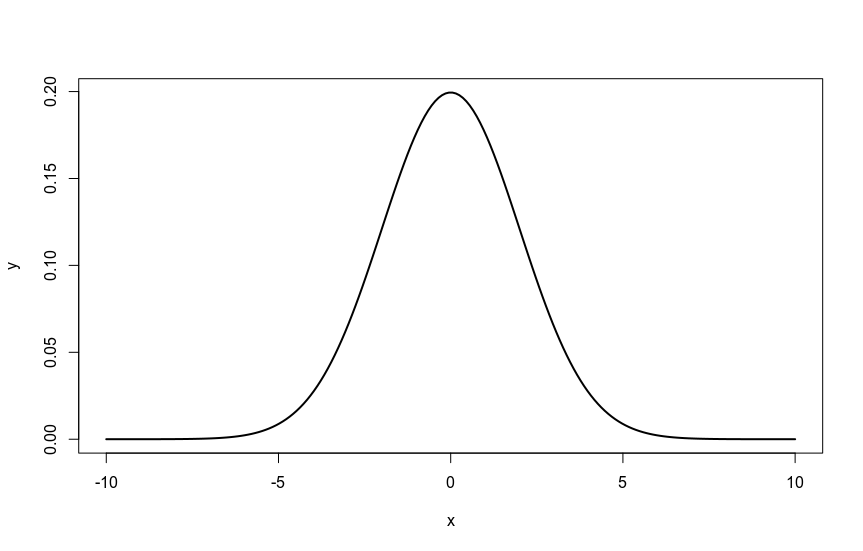
The normal distribution has a bell shape, is also called Gaussian – after the famous mathematician who made a fundamental contribution to this field – and is symmetrical about its mean. It extends indefinitely in both directions, but most of the area – that is, the probability – is collected around the mean. The curve appears to change shape at two points, which we call inflection points, and which coincide with a distance of one standard deviation more and less than the mean.
I generate with a couple of lines in R the characteristic shape of this distribution:

Visualizing the “normality” of our data
R offers several tools to evaluate the deviation of a distribution from a theoretical normal distribution.
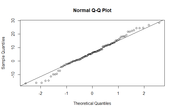
One of these is the qqnorm() function, which creates a plot of the distribution as a function of the theoretical normal quantiles (qq=quantile-quantile):
qqnorm(variable) qqline(variable)
I verify this with an example by generating a normal distribution:
x<- rnorm(100,5,10) qqnorm(x) qqline(x)
The result is this, and as you can see, we have visual confirmation of the substantial normality of the distribution:

Transforming the data
When the asymmetry of a distribution depends on the fact that a variable extends over various orders of magnitude, we have an easy way to make our distribution symmetrical and similar to a normal distribution: transform the variable into its logarithm:
qqnorm(log10(variable)) qqline(log10(variable))
But how do I calculate the central tendency in this case? If I use something like mean(log10(variable)), I no longer have the unit of measurement… To recover it, I can use the antilogarithm, i.e., calculate: 10^result. However, it must always be kept in mind that this is the geometric mean.
Good: we have our dataset and we have verified that the distribution is reasonably similar to a normal distribution. It’s time to find some practical applications to put our new knowledge to use!
The empirical rule
The empirical rule is one of the pillars of statistics. Without going into too much theoretical detail, the gist is this: the percentages of data from a normal distribution within 1, 2, and 3 standard deviations from the mean are approximately 68%, 95%, and 99.7%. It is a rule of such importance and common use that it is better to rewrite it with greater emphasis…
THE EMPIRICAL RULE
The percentages of data from a normal distribution within
1, 2, and 3 standard deviations from the mean
are approximately
68%, 95%, and 99.7%.
Standardizing is useful (and beautiful…). The Z score.
The standardized normal distribution is a normal distribution with a zero mean and standard deviation (or standard deviation, as the English speakers say) of one.
* In the blog, I use the two terms “standard deviation” and “standard deviation” interchangeably… since they express the same concept and are both commonly used.
That is, with:
\( \mu=0 \ \sigma=1 \ \)Any normal distribution can be converted into a standardized normal distribution by setting the mean to zero and expressing the deviations from the mean in units of standard deviation, what the English speakers very effectively call Z-score.
A Z-score measures the distance between a data point and the mean, using standard deviations. Therefore, a Z-score can be positive (the observation is above the mean) or negative (below the mean). A Z-score of -1, for example, will indicate that our observation falls one standard deviation below the mean. Obviously, a Z-score equal to 0 is equivalent to the mean.
The Z-score is a “pure” value, so it provides us with a “measure” of extraordinary effectiveness. In practice, it is an index that allows me to compare values between different distributions (as long as they are “normal,” of course), using a “standard” measure.
The calculation, as we have seen, is almost trivial: simply divide the deviation by the standard deviation:
Under these conditions, we know that approximately 68% of the area under the standardized normal curve is within 1 standard deviation from the mean, 95% within two, and 99.7% within three.
That is:
To find the probabilities – that is, the areas – for problems involving the normal distribution, the value X is converted into the corresponding Z-score:
\( Z = \frac{X-\mu}{\sigma} \ \ \)Then the value of Z is looked up in the tables and the probability under the curve between the mean and Z is found.
Seems difficult? It’s very easy, and very fun. And with R, or with the TI-83, it’s really a breeze!
The importance of the Z-score also lies (and especially) in its extreme practical utility: it allows, in fact, to usefully compare observations drawn from populations with different means and standard deviations, using a common scale. This is why the process is called standardization: it allows comparing observations between variables that have different distributions. Using the table (or the calculator or the computer) we can quickly calculate probabilities and percentiles, and identify any extreme values (outliers).
Since sigma is positive, Z will be positive if X>mu and negative if X<mu. The value of Z represents the number of standard deviations the value is above or below the mean.
Let’s do a quick example
I have observations of some phenomenon that have a mean value of 65:
\( \mu = 65 \ \)The standard deviation is 10:
\( \sigma = 10 \ \)And I observe a value of 81 :
\( X = 81 \\ \)The value of the Z-score is calculated in a moment:
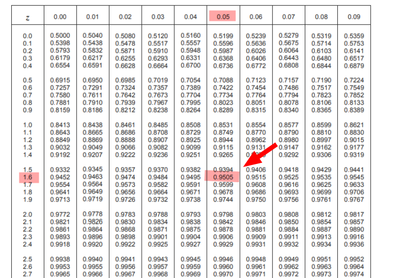
\( Z= \frac{X – \mu}{\sigma} = \frac{81 – 65}{10} = \frac{16}{10} = 1.6 \ \)The observed value, on a standard scale, falls 1.6 standard deviations above the mean. To understand, therefore, what percentage of observations result below the observed value, I just need to take the table:

As noted, by crossing my z value: 1.6 at the 0.05 level I find the value 0.9505, which is equivalent to saying that 95.05% of the observed values are less than 81.
Obviously, I could have obtained the value in R without using the table, simply with:
pnorm(1.6)
For those using Python:
from scipy.stats import norm p = norm.cdf(1.6) print(p)
And now the fun part: let’s do some practical examples!
Example 1
What is the probability of an event with a Z-score < 2.47 ?
I take the table and see that 2.47 = 0.9932.
Therefore, 99.32% of the values are within 2.47 standard deviations from the mean.
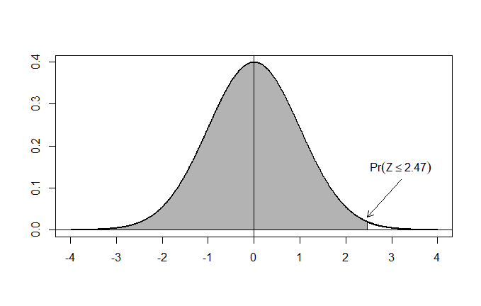
Graphically representing the situation, what I am asked to do is to find the area of the gray surface, that is, the area under the curve to the left of the point with abscissa Z=2.47:

In R, the calculation is very simple. All I have to do is type:
pnorm(2.47)
The pnorm() function allows us to obtain the cumulative probability curve of the normal distribution. In other words, it allows us to calculate the relative area (remembering that the total area is 1) under the curve, from the given value of Z to +infinity or -infinity.
By default, R uses the lower tail, i.e., it finds the area from -infinity to Z.
To compute the area between Z and +infinity, I just need to set lower.tail=FALSE.
Example 2
What is the probability of a Z-score value > 1.53 ?
From the table, I find the value 0.937, so I deduce that 93.7% of the values are below a Z-score of 1.53.
So, to find out how many are above: 100-93.7 = 6.3%
In R, all I have to do is type:
1 - pnorm(1.53)
Example 3
What is the probability of “drawing” a random value of less than 3.65, given a normal distribution with a mean = 5 and a standard deviation = 2.2 ?
I immediately find the Z-score for the value 3.65:
\( Z= \frac{3.65 – 5}{2.2} = \frac{-1.35}{2.2} \simeq -0.61 \ \ \)I look for this value in the table: 0.2709. Therefore, there is a 27.09% probability that a value less than 3.65 will “come out” of a random selection with a mean of 5 and a standard deviation of 2.2.
If I wanted to use a scientific calculator, with the TI83 I would just have to type:
normalcdf(-1e99,3.65,5,2.2)
While with a Casio fx I would just have to follow these steps:
MENU STAT DIST NORM Ncd Data: Variable Lower: -100 Upper: 3.65 sigma: 2.2 mu: 5 EXECUTE
The result is obviously slightly different from that obtained from the table, because in the table I rounded the value of the division (3.65-5)/2.2 to -0.61, omitting the remaining decimal part…
Example 4: finding probabilities between 2 Z-scores
This is the most fun case of all. Actually, just find the 2 probabilities and subtract…
What is the probability associated with a value between Z=1.2 and Z=2.31 ?
I think of my normal curve: first I find the area to the left of Z2. Then I find the area to the left of Z1. Then I subtract the two values to find the area between the two, which is the probability sought.
Or I use R and simply write:
pnorm(2.31)-pnorm(1.2)
and the result, in this case 10.46%, is found in a moment!
Wait, but what if I wanted to calculate the value of Z starting from a cumulative probability? Just use the inverse function of pnorm() which in R is qnorm(). For example, to find the value of Z with an area of 0.5, I type:
qnorm(0.5)
and I will get the result, which is clearly 0 (the mean of a standardized normal has a value of 0 and the mean divides the normal into two equal areas…).
For those using Python, the code is:
from scipy.stats import norm q = norm.ppf(0.5) print(q)
Chebyshev’s inequality
The most important characteristic of Chebyshev’s inequality is that it applies to any probability distribution of which the mean and standard deviation are known.
Dealing with a distribution of unknown type or certainly not normal, Chebyshev’s inequality comes to our aid, stating that:
If we assume a real positive value k, the probability that the random variable X has a value between:
is greater than:
\( 1 – \frac{1}{k^{2}} \ \)In other words: suppose we know the mean and standard deviation of a set of data, which do not follow a normal distribution. We can say that for every value k >0 at least a fraction (1-1/k2) of the data falls within the interval between:
\( \mu \ – \ k \sigma \ e \ \mu \ + \ k \sigma \\)As always, an example is useful to clarify everything. I take an example dataset…the average salaries paid by U.S. baseball teams in 2016:
| Team | Salary (\$M) |
|---|---|
| Arizona Diamondbacks | 91,995583 |
| Atlanta Braves | 77,073541 |
| Baltimore Orioles | 141,741213 |
| Boston Red Sox | 198,328678 |
| Chicago Cubs | 163,805667 |
| Chicago White Sox | 113,911667 |
| Cincinnati Reds | 80,905951 |
| Cleveland Indians | 92,652499 |
| Colorado Rockies | 103,603571 |
| Detroit Tigers | 192,3075 |
| Houston Astros | 89,0625 |
| Kansas City Royals | 136,564175 |
| Los Angeles Angels | 160,98619 |
| Los Angeles Dodgers | 248,321662 |
| Miami Marlins | 64,02 |
| Milwaukee Brewers | 51,2 |
| Minnesota Twins | 99,8125 |
| New York Mets | 128,413458 |
| New York Yankees | 221,574999 |
| Oakland Athletics | 80,613332 |
| Philadelphia Phillies | 91,616668 |
| Pittsburgh Pirates | 95,840999 |
| San Diego Padres | 94,12 |
| San Francisco Giants | 166,744443 |
| Seattle Mariners | 139,804258 |
| St, Louis Cardinals | 143,514 |
| Tampa Bay Rays | 60,065366 |
| Texas Rangers | 158,68022 |
| Toronto Blue Jays | 131,905327 |
| Washington Nationals | 142,501785 |
The mean is: 125.3896
The standard deviation: 48.64039
Chebyshev’s inequality
\( 1 – \frac{1}{k^{2}} \ \)tells us that at least 55.56% in this case is in the interval:
\( (\mu − 1.5\sigma, \mu + 1.5\sigma)= (52.42902, 198.3502) \ \ \)