Multiple Regression Analysis, Explained Simply

The phenomena we observe and wish to study in order to deepen our understanding rarely present themselves so simply as to be defined by only two variables: one predictive (independent) and one response (dependent).

Therefore, while simple linear regression analysis holds fundamental theoretical importance, in practice it provides little more information than simply studying the correlation coefficient.

This is why, in scientific literature, multiple regression plays a predominant role, offering a comprehensive set of tools to explain the variation of our dependent variable for each predictive variable present in the model, as well as for the interactions among the independent variables.

The Multiple Regression Equation

Let’s start with the multiple regression equation, which is essentially an “expansion” of the simple linear regression equation and has this general form:

\( y = a_1 x_1 + a_2 x_2 + … + a_i x_i + b \\ \)

where
y is the response variable (note: it is single)
a_1,a₂…a_i are the regression coefficients for the predictive variables
x₁,x₂…x_i are the predictive variables
b is the intercept (also single)

What Insights Can I Gain?

First, I need to understand how significantly my predictive variables, when combined, are related to the dependent variable, and what proportion of the outcome is explained by the combination of predictive variables used in the model.

Next, I need to understand how each predictive variable is linked to the dependent variable, while controlling for the other independent variable (assuming, for simplicity, that there are only two predictive variables).

Then, I must determine which of my two predictors has the strongest impact in estimating the dependent variable.

These and many other insights can be obtained through the tools provided by multiple regression analysis, and these initial steps already demonstrate the power and practical utility of this technique.

A Few Prerequisites to Start

Multiple regression analysis is a powerful and widely used technique, but to use it correctly, certain fundamental assumptions must be met:

1. The dependent variable must be measured on an interval or ratio scale, and the predictive variable must also be interval/ratio or dichotomous.
2. There must be a linear relationship between the predictive variable and the dependent variable.
3. All variables in the regression analysis should exhibit a normal distribution.
4. The predictive variables should not be highly correlated with each other (known as multicollinearity). Prediction errors should be independent of each other.
5. It is assumed that heteroscedasticity is present. In other words, the errors in predicting Y should be approximately the same in magnitude and direction across all levels of X.

How to Proceed Practically?

My suggestion for gaining proficiency is to proceed step by step. Here’s my recommended approach:

1. Plot scatterplots for each predictive variable against the response variable to assess the presence of a correlation.
2. Calculate the multiple regression equation.
3. Verify that the assumptions of normality and homoscedasticity are met.
4. Analyze the coefficient of determination.

For each of these steps, R proves to be, as usual, a highly reliable companion, capable of providing the necessary calculations with just a few commands.

Let’s Get Started!

Let’s start R and dive into a practical example, keeping it as simple as possible. We’ll only be scratching the surface here. The goal is to lay the foundation for exploring a vast topic, leaving the reader to delve deeper. So, without further ado, let’s pick a sample dataset.
Among others, R provides Longley’s Economic Regression Data, which I’ll use here.
What is it? It’s a data frame containing seven economic variables from 1947 to 1962.

Let’s open R Studio, load the dataset, and take a first look:

data(longley) dim(longley) head(longley)

Now, let’s examine the metrics. For our example, we’ll use the number of employed individuals as the response variable and the Gross National Product (GNP) and population as the independent predictive variables.

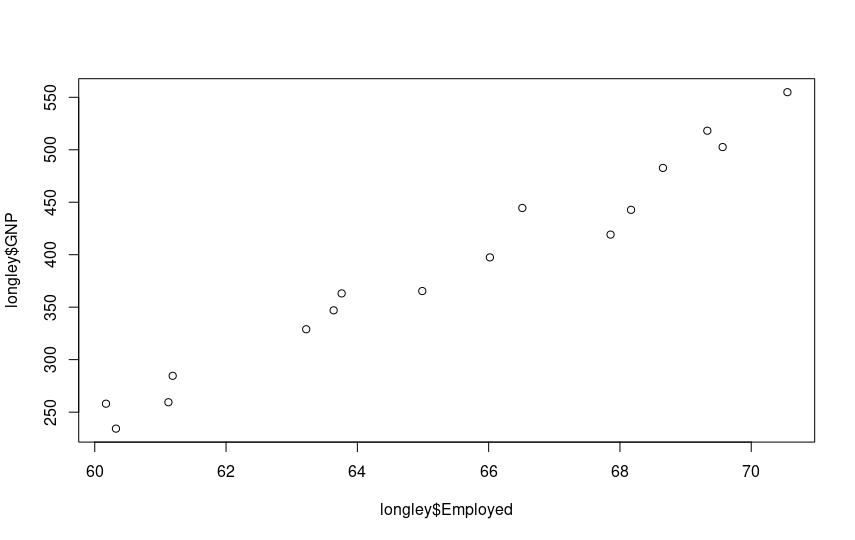
Here’s how the scatterplots look:

plot(longley$Employed, longley$GNP)

plot(longley$Employed, longley$Population)

The growing linear correlation is evident. Let’s proceed with multiple regression. We already know the command: it’s lm(). The syntax for multiple predictor variables is as follows:

regression = lm(Employed ~ GNP + Population, data=longley)
summary(regression)

The result is a wealth of information!

Call:
lm(formula = Employed ~ GNP + Population, data = longley)

Residuals:
     Min       1Q   Median       3Q      Max 
-0.80899 -0.33282 -0.02329  0.25895  1.08800 

Coefficients:
            Estimate Std. Error t value Pr(>|t|)    
(Intercept) 88.93880   13.78503   6.452 2.16e-05 ***
GNP          0.06317    0.01065   5.933 4.96e-05 ***
Population  -0.40974    0.15214  -2.693   0.0184 *  
---
Signif. codes:  0 ‘***’ 0.001 ‘**’ 0.01 ‘*’ 0.05 ‘.’ 0.1 ‘ ’ 1

Residual standard error: 0.5459 on 13 degrees of freedom
Multiple R-squared:  0.9791,	Adjusted R-squared:  0.9758 
F-statistic: 303.9 on 2 and 13 DF,  p-value: 1.221e-11

First, let’s note the p-value of the F-Statistic. It’s very small (1.211e-11), highly significant. Therefore, at least one of our predictor variables is statistically significantly related to the outcome variable. So, let’s proceed.

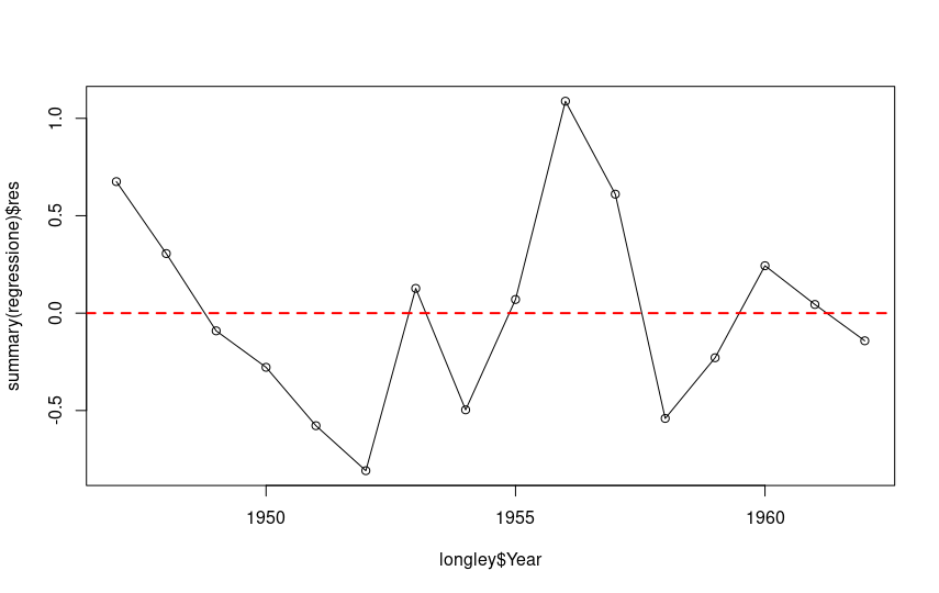
Let’s also plot the residuals:

plot(longley$Year, summary(regression)$res, type='o')
abline(h=0, lty=2, col="red", lwd=2)

Ideally, the sum of the residuals, or the differences between the actual and predicted values, should tend toward zero, or at least be as low as possible. A look at this section of the summary output tells us that this condition is met in this case:

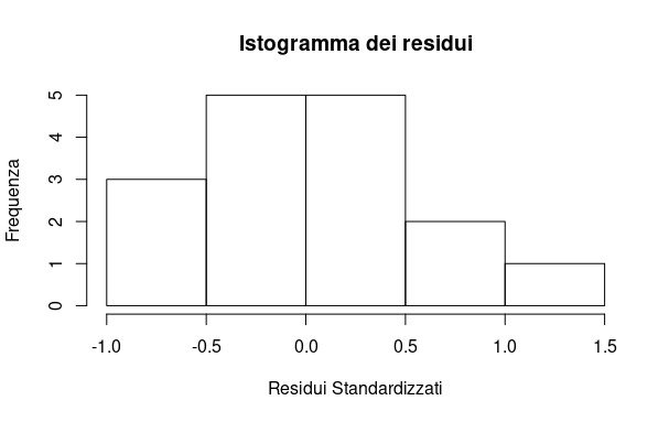
Let’s visually check the assumption of normality for the residuals:

hist(resid(regression),main='Histogram of Residuals',xlab='Standardized Residuals',ylab='Frequency')

The resulting plot shows that the normality assumption is met:

It’s time to look in detail at what the summary output of our regression tells us.

The median is close to zero, and the residuals are approximately normally distributed. So we can proceed.

The values of the coefficients for our two predictor variables and the intercept can be found in our output:

The regression line is thus:

\( \\ y = 0.06317x_1 – 0.40974 x_2 + 88.9388 \\ \)

We pay attention to the p-values concerning the slope coefficients. The output shows that our independent variables are significant in predicting the value of the dependent variable, with p-values below the standard 0.05 threshold. The gross national product even has a value below the 0.001 level. We can therefore reject the null hypothesis (predictor variables are not significant) and validate our model, observing that GNP is the most “reliable” element for estimation compared to the population. The asterisk notation in the output is also very useful, giving us a quick visual insight into the results.

We can also ask R to calculate the confidence interval for our model with the command:

confint(regression)

In our example, we obtain this output:

                  2.5 %       97.5 %
(Intercept) 59.15805807 118.71953854
GNP          0.04017053   0.08617434
Population  -0.73841447  -0.08107138

How valid is my model?

At this point, a key player we have encountered in previous articles comes into play: the coefficient of determination, or r².

It provides essential information about how close the data points are to our regression line. In practical terms, it indicates what percentage of the “movements” in the dependent variable are explained by our predictor variables. The value is standardized between 0 and 1, and it’s clear that our model becomes more useful the closer this value gets to 1.

R, as always remarkable, has already provided us with this useful value in the output. Here it is:

Okay, but what is the Adjusted R-squared value? This is the value to consider, as it solves a paradox with the r² value, which always increases as the number of variables increases (even if those variables aren’t significant at all). The adjusted R-squared corrects this anomaly, providing a perfectly usable value (always lower than R-squared).

Final summary

I’ll keep it short: a high R-squared value and a very low, close-to-zero residual value indicate a good model.

This is not everything; in fact, it’s just the beginning. But it’s the first step in mastering a tool like multiple linear regression analysis, which has great practical utility. I hope to leave you curious to explore further and go beyond (and below are some useful free online resources). Good luck!

---

Free resources for further learning

• You can freely download the second edition of the excellent book “An Introduction to Statistical Learning” by Gareth James and others (Springer). It’s a hefty PDF file of over 600 pages, in English.
• You can access the “Cookbook for R” site, which also has sections dedicated to regression analyses.
• On the R-bloggers website, you can find articles and insights on any statistical and ML topic, with examples and R code.