Decision Trees are a type of machine learning algorithm that uses a tree structure to divide data based on logical rules and predict the class of new data. They are easy to interpret and adaptable to different types of data, but can also suffer from problems such as overfitting, complexity, and imbalance.
Let’s understand a bit more about them and examine a simple example of use in R.

Decision Trees: A Powerful Classification Tool

Imagine you’re a doctor and you need to diagnose a patient’s illness based on some symptoms. How would you decide which disease the patient has? You could use your experience, your intuition, or consult manuals. Or you could use an algorithm that guides you step by step to choose the most likely diagnosis, based on the data you have available. This algorithm is called a Decision Tree.

A Decision Tree is a graphical structure that represents a series of logical rules for classifying objects or situations.
Each node of the tree represents a question or condition, which divides the data into two or more homogeneous subgroups.
Each branch represents a possible answer or action, which connects one node to another node or to a leaf.
The initial node is called the root, and it’s the starting point of the tree.
The final nodes are called leaves, and they are the end points of the tree.
Each leaf corresponds to a class, that is, a category to which the object or situation to be classified belongs.

Decision Trees are widely used in scientific, technological, medical, economic, and social fields because they have several advantages:

• They are easy to interpret and communicate, even to non-experts.
• They are flexible and can adapt to different types of data, both numerical and categorical.
• They are robust and can handle incomplete, noisy, or inconsistent data.
• They are efficient and require little time and memory to be built and applied.

However, Decision Trees also have some disadvantages:

• They can be unstable, that is, sensitive to small variations in the initial data, and therefore produce very different trees.
• They can be complex, that is, have many nodes and branches, and thus lose clarity and accuracy.
• They can be imbalanced, that is, favor some classes over others, and therefore be unrepresentative of reality.

To overcome these problems, there are various techniques for optimization and validation of Decision Trees, which allow improving their performance and evaluating their reliability.

A Simple Example of a Decision Tree in R

To better understand how Decision Trees work, let’s look at a practical example in R language.

For our example, we’ll use the iris dataset, which contains measurements of sepal length and width and petal length and width of 150 iris flowers, belonging to three different species: setosa, versicolor, and virginica. Our goal is to build a Decision Tree that allows us to classify an iris flower based on its species, using its measurements as explanatory variables.

First, let’s load the iris dataset and the rpart library, which allows us to create Decision Trees in R.

# Load the iris dataset
data(iris)
# Load the rpart library
library(rpart)
# Set the seed for reproducibility
set.seed(123)
# Randomly extract 80% of the rows from the dataset
train_index <- sample(1:nrow(iris), 0.8*nrow(iris))
# Create the training dataset
train_data <- iris[train_index, ]
# Create the test dataset
test_data <- iris[-train_index, ]

Now, we’re ready to build our Decision Tree, using the rpart function. This function requires some parameters:

• The formula, which specifies the variable to be classified (in this case, Species) and the explanatory variables (in this case, all the others).
• The dataset, which contains the data to be used to build the Decision Tree (in this case, train_data).
• The method, which specifies the type of classification to be used (in this case, class, which indicates a categorical classification).

# Build the Decision Tree
tree <- rpart(formula = Species ~ ., data = train_data, method = "class")

To visualize our Decision Tree, we use the plot function, which allows us to draw the graphical structure of the tree, and the text function, which allows us to add labels to the nodes and branches.

# Visualize the Decision Tree
plot(tree, uniform = TRUE, branch=0.8)
text(tree, all=TRUE, use.n = TRUE)

The result is as follows:

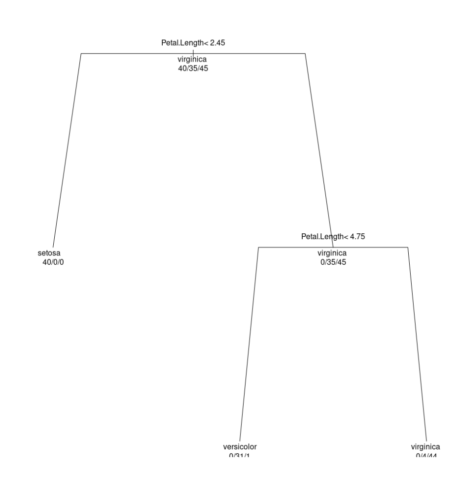
How can we interpret this simple Decision Tree? Let’s start from the root, which is the node at the top. This node tells us that the most important variable for classifying an iris flower is the petal length (Petal.Length). If the petal length is less than 2.45 cm, then the flower is of the setosa species. If instead the petal length is greater, we need to consider whether the petal length is less than or equal to 4.75 cm. If it’s less, then the flower is of the versicolor species. If instead the petal length is greater than 4.75 cm, then the flower is of the virginica species.

How to Evaluate the Accuracy of a Decision Tree

To evaluate the accuracy of a Decision Tree, we need to compare the classes predicted by the tree with the actual classes of the test data. To do this, we use the predict function, which allows us to apply the Decision Tree to the test data and obtain the predicted classes.

# Apply the Decision Tree to the test data
pred_class <- predict(tree, newdata = test_data, type = "class")

Then, we use the table function, which allows us to create a contingency table between the predicted classes and the actual classes.

# Create the contingency table
table(pred_class, test_data$Species)

The result is as follows:

	setosa	versicolor	virginica
setosa	10	0	0
versicolor	0	13	0
virginica	0	2	5

This table shows us how many times the Decision Tree correctly predicted or misclassified the species of an iris flower. For example, the cell in the top left tells us that the Decision Tree correctly predicted that 10 flowers were of the setosa species. The cell at the bottom center tells us that the Decision Tree wrongly predicted that 2 flowers were of the virginica species, when in fact they were of the versicolor species.

To calculate the accuracy of a Decision Tree, we need to divide the number of correct predictions by the total number of predictions. In this case, the accuracy is:

\( \frac{10 + 13 + 5}{10 + 13 + 5 + 2} = \frac{28}{30} = 0.93\\ \)

This means that our Decision Tree correctly predicted the species of an iris flower in 93% of cases. This is a good result, but it could be improved with some optimization techniques, such as pruning or variable selection.

Pruning is a technique that consists of reducing the complexity of a Decision Tree by eliminating some nodes or branches that do not significantly contribute to accuracy. This can prevent the problem of overfitting, which is when the Decision Tree adapts too much to the training data and loses the ability to generalize to the test data.

Variable selection is a technique that consists of choosing the most relevant variables for classification, eliminating those that are irrelevant or redundant. This can improve the accuracy and clarity of the Decision Tree, reducing the number of questions or conditions to consider.

What is Overfitting?

Overfitting is a problem that occurs when a machine learning model adapts too much to the training data, and fails to generalize well to new data. This means that the model memorizes the specific characteristics and noise of the training data, but fails to capture the general trend of the data. As a result, the model has high accuracy on the training data, but low accuracy on the test or validation data. Overfitting can be caused by excessive complexity of the model, insufficient training data, or too long training.

Brief Overview of Other Classification Algorithms

There are countless other classification algorithms, such as logistic regression, k-nearest neighbor, support vector machine, and neural networks. These algorithms are based on principles different from Decision Trees, such as probability function, distance, margin, or non-linear transformation of data. Some of